Utilization

Every software organization faces pressure to maximize utilization. There is pressure to fill every sprint, assign every engineer, and keep every slot in the pipeline occupied to maximize output. I will present a simple visual analogy of two different roller coaster designs and contrast their performance to demonstrate why this instinct is not merely suboptimal but can even be catastrophic.

I modeled two systems processing identical work through identical constraints. They demonstrate two extremes of a continuum from excess slack to 100% utilization.

The Analogy

Imagine a roller coaster track as your software delivery pipeline. Each passenger is a feature, enhancement, or bug fix. The boarding station is your deployment process. The track itself represents all the work between inception and release: design, development, code review, QA, staging, and deployment.

System A: Two Short Trains (“Slack in the System”). Two independent trains of 5 cars each circle the track. Each train arrives at the station, unloads passengers, loads 5 new ones, and departs. The other train continues circling while the first is boarding. The track is roughly 89% empty at any given time.

System B: One Continuous Train (“Full Utilization”). A single train of 103 cars fills the entire track end to end. It advances 5 cars at a time, pauses to unload and reload, then advances again. Every inch of track is occupied. Utilization is 100%. There is no slack anywhere in the system.

Measured Performance

The following metrics were computed directly from the running simulations:

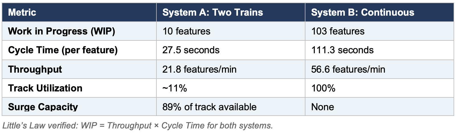
On the surface, System B looks like the clear winner: 2.6× the throughput, 100% utilization, no idle capacity. Many managers would look at these numbers and choose System B without hesitation. They would be making a terrible mistake.

Kingman’s Approximation: Wait Time Increases with Utilization

In 1961, Sir John Kingman published an approximation for the average waiting time in a single-server queue. The formula, known as the Kingman or VUT equation, is one of the most important results in operations research:

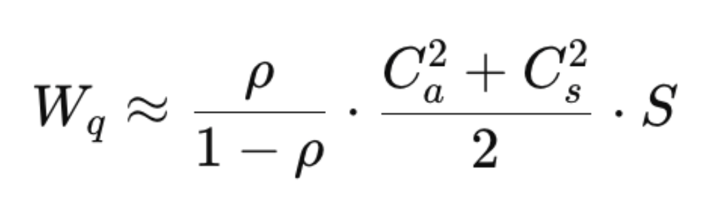
• Wq = wait time. That’s how much time things sit idle as they move through the system.
• ρ = utilization percentage.
• Ca^2 = squared coefficient of variation of the arrival process
• Cs^2 = squared coefficient of variation of the service process (service time is the amount of time spent on effort as opposed to waiting)
• S = service time (touch time or effort)

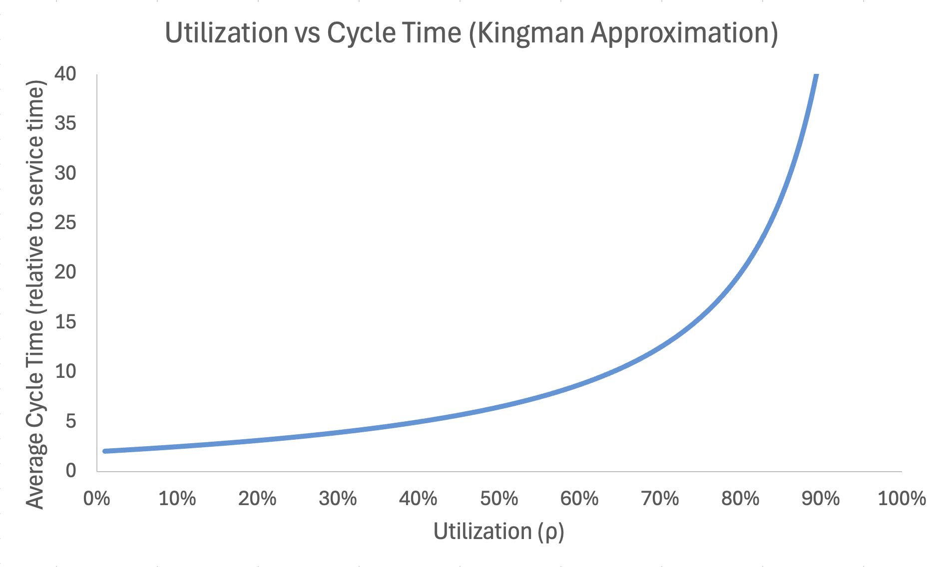
The critical term is ρ/(1–ρ). This is not a linear relationship. It is a hyperbola that approaches infinity as utilization approaches 100%:

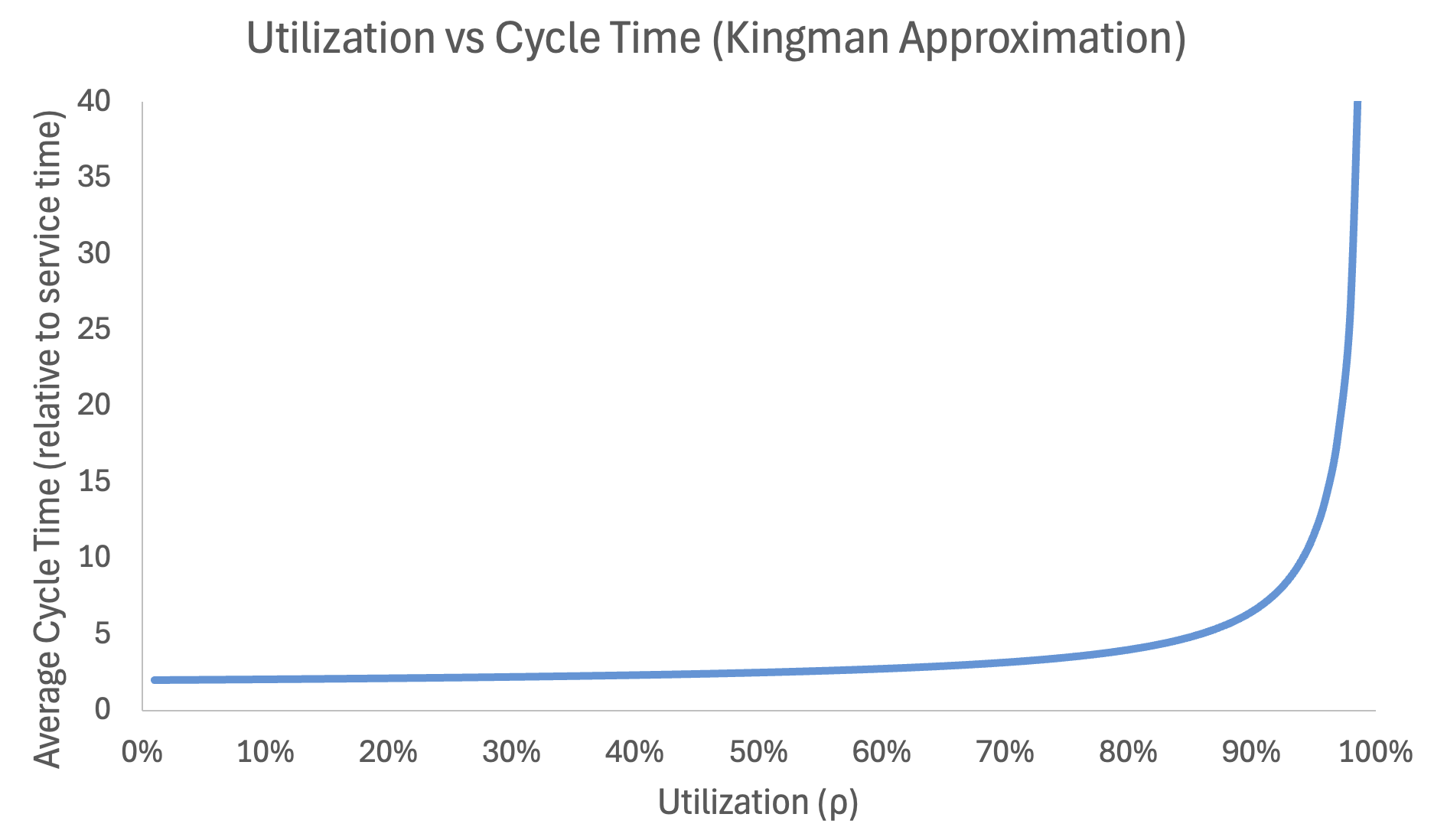
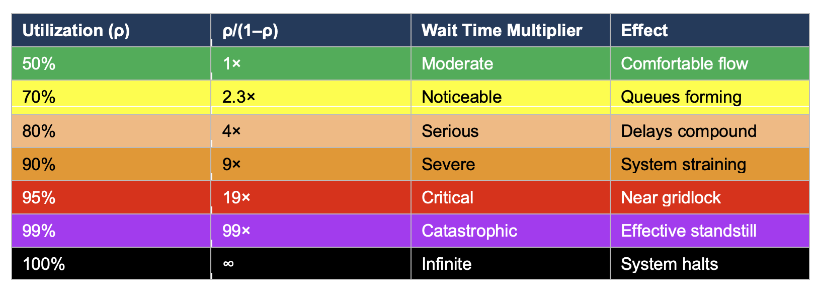
In fact, the more variability there is in a system, the less utilization the system can tolerate before wait times start to explosively increase. Software development is a high variability environment.

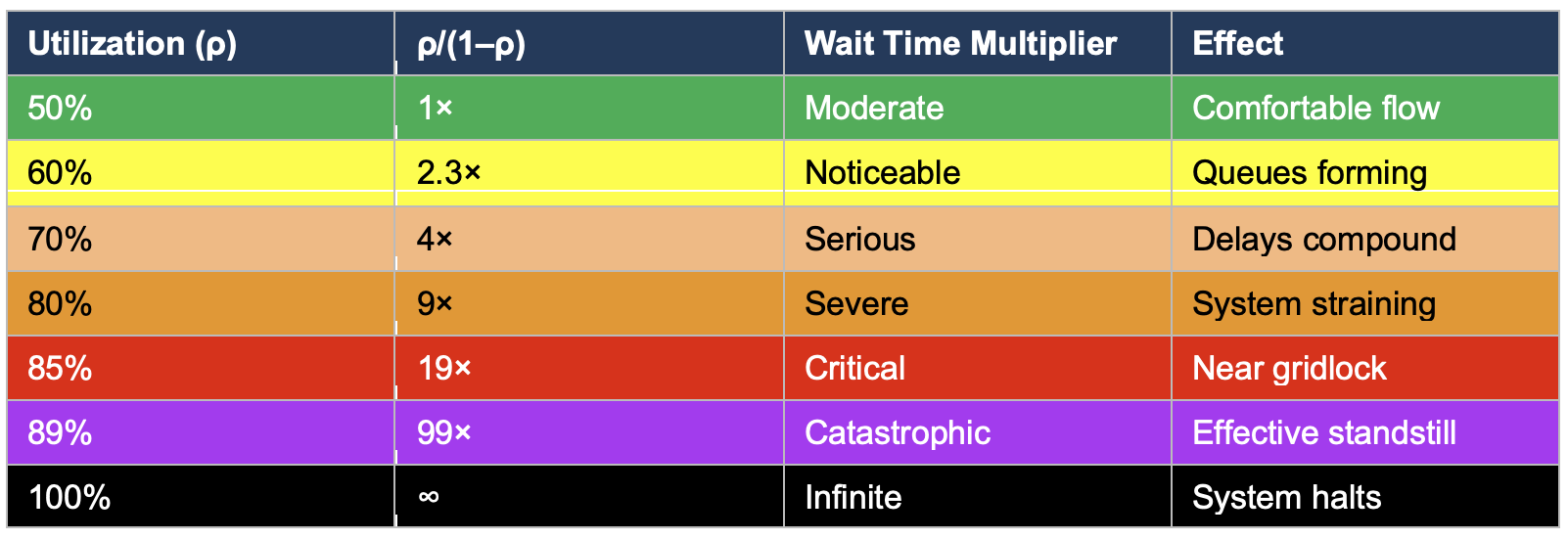
Kingman’s Approximation with High Variability

This table alone should end the conversation about full utilization. But it gets worse. The formula also multiplies by the variability terms (c²ₐ + c²ₛ)/2. In manufacturing, these coefficients might be 0.5 or less—machines are predictable. In software development, they are routinely above 1.0 and often above 2.0. Some features take a day while others take a quarter. Requirements are constantly changing before anything is delivered. The team is interrupted with new ideas or changes mid-sprint. Dependencies fail to deliver and work gets blocked. Key engineers get sick. Production incidents hijack capacity. Someone in sales has promised a customer something without talking to anyone, and the team is redirected to estimating a complex product delivery that the current architecture doesn’t even support.

The curve in software development looks more like this when we adjust arrivals and service time variables to values that represent high variability: (1.5 – 2.0):

Kingman’s formula does not say that high utilization is “suboptimal.” It says that in a system with variability, as utilization approaches 100%, wait times approach infinity. This is not a tendency or a risk. It is a mathematical certainty.

The Variability Problem

Return to the roller coaster. System B has 103 cars filling every inch of track. Now imagine an unexpected event: a passenger gets sick. A car needs unscheduled maintenance. A section of track needs emergency inspection. In the language of software development: a critical production bug, an infrastructure outage, a key engineer’s departure, a security vulnerability, a sudden change in priorities from the board. These things are all examples of variability. In software development, variability is high.

The problem with choosing the high utilization = high throughput system is variability. Unforeseen yet completely expected events will destroy what was envisioned as a perfectly efficient, low-cost, high-output system.

• The entire train stops. All 103 cars are coupled. One blockage halts everything. There is no way to route around it because every inch of track is occupied.
• The queue grows without bound. During the stoppage, new features keep arriving (the business doesn’t stop having ideas). With zero slack, there is nowhere to absorb them. The backlog explodes.
• Recovery takes longer than the disruption. After the blockage clears, the system doesn’t instantly return to steady state. It must work through the accumulated queue, still at 100% utilization, which Kingman tells us means wait times are already infinite. The system never truly recovers—it lurches from crisis to crisis.
• Every subsequent disruption compounds the last. Because there is no slack to absorb the first shock, the system is still degraded when the second one arrives. Delays cascade. Commitments slip. Teams begin cutting corners to catch up, introducing more defects, which create more disruptions.
• Technical debt. As teams begin to cut corners to catch up, technical debt begins to build. The more technical debt in the code base, the probability that any work item becomes more complex increases. This compounds and further increases cycle time.

It will take so long for work to pass through the system that by the time it arrives, customers and stakeholders are furious. The long cycle times will destroy any hope of valuable feedback during product design and development. The long waits mean that wait times will further increase as stakeholders, knowing they face a long wait to receive results, pack in even more scope and engage in more self-destructive behavior to speed delivery.

System A: Graceful Degradation

Slack in the system is capacity reserved for speed. That reserved capacity is a buffer against variability.

• One train stops; the other keeps moving. The independent trains provide redundancy. Half the system continues delivering while the other handles the disruption.
• 89% of the track is empty. This is not waste—it is a buffer that absorbs variability. An emergency feature can board the next available train without displacing anything. A priority change reorders the queue, not the train.
• Recovery is fast. Because the system normally operates well below capacity, it returns to steady state quickly after a disruption. The queue doesn’t explode because there was room to absorb the shock.
• Disruptions are isolated. A problem with one train does not propagate to the other. In software terms: a team dealing with a production incident doesn’t block the team shipping a planned feature.

Overhead costs are reduced, work flows more quickly. Feedback loops are achievable.

The Temptation of Full Utilization

There will always be a nagging voice in any manager’s head saying that idle people are scamming you. You will imagine they are watching television, going to the gym, or otherwise not available. In a few cases, you might be correct. In a work from home world, those things can happen. However, the larger percentage of people will not do this to you. They will not be literally idle. They will busy themselves with learning activities and valuable conversations. They might start cleaning up messes that were left behind by previous work. This “idle” time isn’t a gang of thieves stealing your money in payment per hour. It is your workers learning, improving, recharging, and making themselves ready for what’s coming next. The cost of the highly utilized system is so high that the cost of people being idle is inconsequential. There is no comparison. You are better off accepting the cost and going for the lower cycle times.

It is tempting to argue that System B might work in specific, controlled circumstances—perhaps for “mechanical” work like regulatory compliance, platform migrations, or well-specified roadmaps where variability is low. This argument fails for three reasons:

• Software variability cannot be eliminated. Even the most “routine” software work contains variability. A “simple” API migration uncovers undocumented behavior. A “straightforward” database upgrade reveals data quality issues. A “predictable” compliance feature requires legal review that takes three weeks instead of three days. The coefficient of variation in software work does not drop below 1.0 even in the most controlled environments. Kingman’s formula with c² = 1.0 and ρ = 0.95 still yields a 19× wait time multiplier.
• External variability is uncontrollable. Even if you could perfectly predict service times (you cannot), you cannot control arrival variability. The CEO will walk in with an urgent request. A competitor will launch a feature that demands a response. A security researcher will disclose a vulnerability. AWS will have an outage. These events do not respect your roadmap.
• The failure mode is not gradual. This is the most dangerous misconception. Managers expect that pushing utilization from 80% to 95% will degrade performance proportionally. Maybe 15% worse. Kingman shows the reality: it goes from 4× wait times to 19×, a fivefold increase from a 15-point change. The system does not slow down gracefully. It hits a cliff and collapses.

Strategic Implications

What to Measure:

• Cycle time, not velocity. Velocity measures how much work enters the system. Cycle time measures how quickly work exits it. An organization with high velocity and high cycle time is just packing the roller coaster—lots of features in progress, few reaching customers.
• WIP limits, not resource allocation. Stop asking “is everyone busy?” and start asking “how many things are in flight?” The former drives you toward System B. The latter drives you toward System A.
• Time to recover, not just uptime. Systems with slack recover from disruptions in hours. Fully utilized systems take weeks. Measure how long it takes to return to normal after an incident.

What to Do

• Cap utilization. This is not a soft target. Kingman’s formula shows that the wait-time curve starts bending sharply above 80% in low variability systems and 60% in high variability systems. Protect the remaining 20–40% as strategic reserve for unplanned work, experimentation, technical debt reduction, and recovery from disruptions.
• Limit WIP ruthlessly. Every feature in progress is inventory. Inventory has carrying costs: context in engineers’ heads, branches that could conflict, dependencies that could break, decisions that go stale. Moving from 103 WIP to 10 eliminates an entire category of coordination failure.
• Resist the utilization reflex. When leadership sees engineers “not busy,” the instinct is to load more work. This is the equivalent of packing more cars onto the track. The short-term optics improve. The system dynamics get worse. Train your organization to understand that slack is the mechanism by which work flows quickly.
• Small batches, independent streams. Structure teams as independent trains that can stop, start, and reroute without blocking each other. Keep batch sizes small (5 cars, not 103) so that each cycle through the station is fast and the cost of any single failure is contained.

Recommendation

There is no context in software development where full utilization in the attempt to maximize throughput is appropriate. Full utilization in a high-variability system is a guarantee of long delivery times, missed dates, high defect rates, and huge overhead costs. Kingman’s Approximation, published in 1961, has been validated across six decades of operations research. It applies to factory floors, hospital emergency rooms, highway traffic, call centers, airports, public transportation, and software delivery pipelines with equal force.

Ship fewer things faster rather than more things slower. Limit work in progress. Availability is not idle capacity. It is your contingency against the inevitable nonsense that happens while trying to deliver a feature. The roller coaster that looks half-empty is delivering passengers to the exit 4x faster. And when someone inevitably throws up, it keeps running.