
Little’s Law is a mathematical relationship that describes how the amount of work in a system, the rate at which work is completed, and the time work spends in the system are connected. Dr. John Little published the formal proof in 1961, and it has been used across many industries ever since. The law does not tell us what to do. It shows us the relationship between tradeoffs.
This is Little’s Law:
L = λ x W

L = Work-In-Process (Items in the system)
λ = Throughput/Departures (Arrivals)
W = Cycle Time (Service Time + Wait Time in Queue)
The law relates three measurable quantities: the rate at which items arrive and depart, the number of items currently in the system, and the average time those items spend there. This relationship holds for any stable system.
The variables of Little’s Law were made L, λ, and W because Little was doing his work in probability, and there is a standard notation for concepts. It can be confusing that the variables don’t match up to the names of the variables we use today:
WIP = Work-in-Process. The amount of work that is currently active in the system. WIP is often counted as a number of items. However, WIP also represents the total amount of unfinished work in the system. A single large, complex item that contains many smaller components still represents substantial WIP.
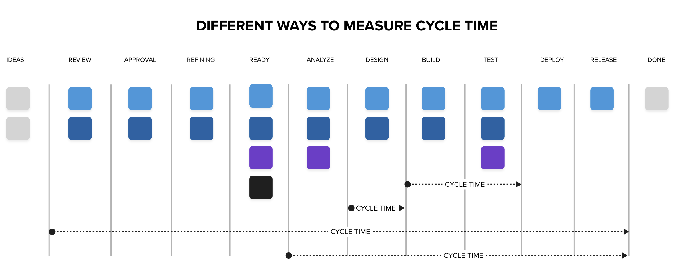
Cycle Time. The elapsed time from the moment that work has begun until it is completed. This is measured between two boundaries such as start and finish. The start and finish boundaries can be defined at the level of the entire value stream or within sub-steps to make delays visible.
Throughput. The number of things that finish moving through the system per unit time.
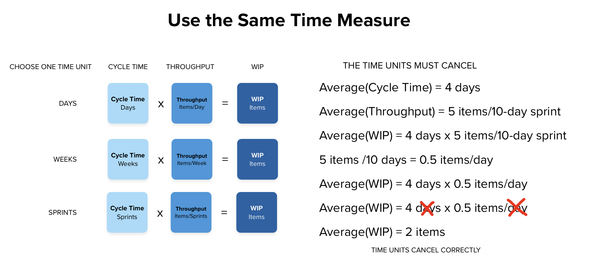
Cycle time can be measured at different boundaries. Because Little’s Law is an equation, once those boundaries are chosen, the time units must be consistent. If throughput is measured per sprint and cycle time per day, the relationship becomes distorted unless the units are converted.
In product development, leaders are rarely concerned with how many items arrive at a system. They want to know when work will finish or how much can be completed by a given date. For that reason, we usually measure departures, because departures define throughput. Under stable conditions, average arrival rate and average departure rate are equal, but departures are what matter when discussing delivery.
The Relationship Between WIP, Throughput, and Cycle Time
Little’s Law is a model built on averages. We can rewrite the equation to:
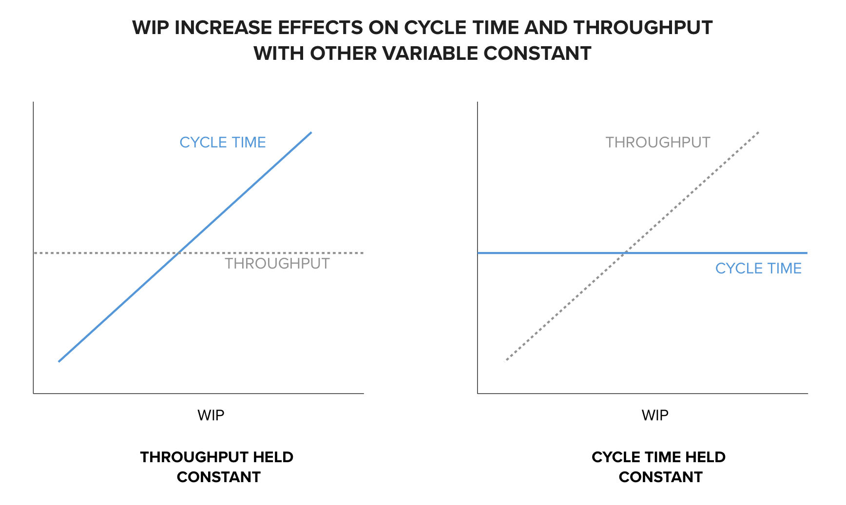
Average(WIP) = Average(Throughput) x Average(Cycle Time)The relationship between these variables is that the average WIP in the system will always be equal to the average throughput multiplied by the average cycle time. If average cycle time increases while throughput remains constant, average WIP must increase. If throughput increases while cycle time remains constant, average WIP must also increase.
Average(Cycle Time) = Average(WIP) / Average(Throughput)These are long-run averages measured over the same time window.
Average cycle time is equal to average WIP divided by average throughput, measured over the same period. If throughput increases while WIP remains constant, cycle time decreases. If WIP decreases while throughput remains constant, cycle time also decreases.
Average(Throughput) = Average(WIP) / Average(Cycle Time)Mathematically, throughput increases if WIP increases while cycle time remains constant, or if cycle time decreases while WIP remains constant. In practice, throughput is constrained by the system’s bottleneck. Increasing WIP beyond that constraint increases cycle time, not throughput.
Keeping cycle time constant while increasing WIP requires additional capacity at the constraint. That capacity has a cost. It increases direct expense and often increases coordination overhead. Throughput does not rise for free.
Little’s Law is a mathematical model, not a management philosophy. It describes a structural relationship that exists whether we acknowledge it or not. It is used in many fields to understand how to improve the flow of value through systems. It is used in manufacturing, transportation, distribution, traffic engineering, and other flow-based disciplines.
How Throughput Can Be Increased
Organizations want higher throughput. Producing more low-value work does not help, but increasing the rate at which valuable ideas move through the system does. For this discussion, we will focus on throughput itself rather than debating the value of individual items.
Throughput is constrained by the system’s bottleneck. The bottleneck is the step whose capacity limits the entire system and where work tends to accumulate. To increase throughput, attention must be focused on the bottleneck. Non-bottleneck steps do not determine overall output. Improvements away from the constraint will not increase total throughput.
Reducing interruptions and quality problems at or before the bottleneck increases its effective capacity. Stabilizing arrivals prevents unnecessary queue spikes that waste constraint capacity. In some cases, work at the constraint can be reorganized. Sequential activities may be separated and performed in parallel. Additional capacity can also be added directly to the constraint. It can also be necessary to throttle what enters the bottleneck. Work that consumes constraint capacity should be limited to items that truly require it.
How Cycle Time Can Be Decreased
Organizations want shorter cycle times. When measured from idea to delivery, cycle time is time-to-market. It defines how frequently new ideas can be released. It sets the cadence of learning.
Cycle time decreases as WIP decreases. Limiting the number of items in progress reduces waiting time in queues. WIP constraints introduce slack into the system, allowing it to absorb variability rather than amplify it. Lower WIP also reduces coordination overhead and the delays created by excessive dependency management.
Reducing WIP decreases cycle time. Throughput may increase if the bottleneck’s effective capacity improves as congestion is reduced. However, throughput remains bounded by the constraint.
If throughput remains constant, reducing WIP must reduce cycle time.
Large batches inflate WIP. Starting one hundred small items at once creates the same load as starting a single large item composed of one hundred smaller parts. In both cases, the system must absorb the same amount of unfinished work. Reducing batch size reduces the amount of work held open at one time, which in turn reduces cycle time.
Little’s Law is a Control Model – Not a Predictive Equation
Little’s Law is not a predictive formula for individual outcomes. It is a control model that shows how WIP, cycle time, and throughput are structurally connected. It allows us to change one variable and observe the effect on the others.
Because the law operates on averages, it does not describe the distribution of outcomes. An average cycle time does not tell us how likely any individual item is to complete within that time.
The Flaw of Averages reminds us that an average does not describe variability. A data set can be widely dispersed around its mean. If a billionaire sits at a table with two ordinary earners, the average net worth appears enormous. When the billionaire leaves, the average collapses. The mean did not describe any individual person at the table.
Similarly, an average cycle time of ten days does not mean most items finish in ten days. The distribution may be skewed. Fewer than half the items might complete within that average.
Predictability using Little’s Law assumes a stable system. A stable system is one in which the average arrival rate equals the average departure rate over time. If arrivals consistently exceed departures, WIP grows without bound and the relationship breaks down. In software development, arrival rates are often volatile. Without deliberate WIP control, the system becomes unstable and averages lose meaning.
Little’s Law is diagnostic, not predictive.
Why Little’s Law Matters
Reducing cycle time creates measurable business effects. When work spends less time in the system, it is less exposed to interruption, reprioritization, or abandonment.
Shorter cycle times reduce business risk because work can be released and evaluated sooner. Feedback arrives earlier, and weak ideas are exposed before large investments accumulate.
Shorter cycle times make the system more responsive to change. When market conditions shift, the organization can adjust direction without unwinding months of in-process work.
Short cycle times reduce the amount of capital tied up in unfinished work. The cost of delay is reduced because benefits are realized sooner.

Last updated 2026-02-17